Implicit Learners

definition overview

A neural network learns a function and runs one way. An implicit learner learns a relation, a set of admissible configurations, and decides at query time which variables are inputs and which are outputs. Inference is root-finding (as in deep equilibrium models), training differentiates through it by the implicit function theorem, and three model families supply the relation: algebraic, equilibrium and diffusion.

Sources: original to this vault (design and analysis); LeCun et al., A Tutorial on Energy-Based Learning, 2006; Bai, Kolter & Koltun, Deep Equilibrium Models, NeurIPS 2019; Mardani et al., A Variational Perspective on Solving Inverse Problems with Diffusion Models, ICLR 2024; St Clere Smithe & Perin, AutoBayes, arXiv:2503.18608 (§6 only); full entries in Bibliography

Theory (CT-ML wiki, for §6): Statistical Game · Bayesian Lens · Open Model

1. The claim: functions versus relations

A regression model learns $f_{\theta }:X\to Y$. Ask it the reverse question, “which $x$ gives this $y$?”, and it has no answer; ask it a question with two right answers, and least squares returns their average. Many problems are not functions:

• inverse kinematics: one hand position, two arm poses (elbow up and down);
• physical laws: $pV=nRT$ determines any one quantity from the other two;
• missing data: whichever columns are missing are the outputs, and that changes per row.

An implicit learner models the joint space of all variables,

$$Z=X\times Y\times U,z=(x,y,u),$$

and learns a residual $r_{\theta }:Z\to {\mathbb{R}}^m$ whose zeros are the admissible configurations:

$$R_{\theta }=\{z\in Z:r_{\theta }(z)=0\}.$$

Nothing in $r_{\theta }$ says which coordinates are inputs. A query says it: it clamps some coordinates (the inputs $X$), leaves others free (the outputs $Y$), and may have latent ones ($U$) that are inferred but not reported. Notation is fixed vault-wide in Channels and Polarity §“Notation”.

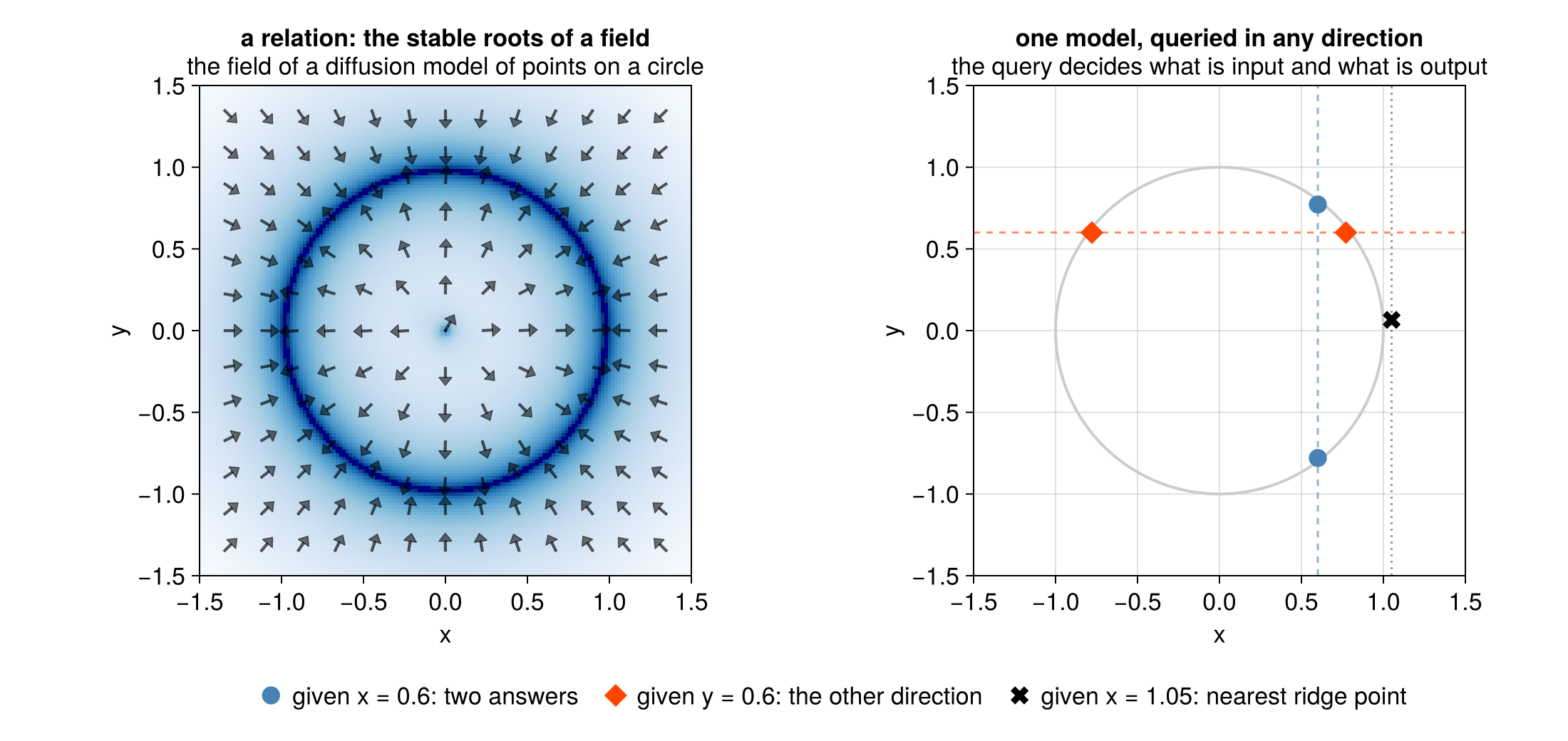
The circle is the smallest example: $Z={\mathbb{R}}^2$, one model, and the questions “given $x=0.6$, find $y$” (two answers), “given $y=0.6$, find $x$” (the same model the other way round) and “given $x=1.05$” (just off the circle). The documentation’s tutorials build this picture, then a trained network, then a robot arm.

2. Inference and training

Inference is root-finding. Given the clamped inputs, solve $r_{\theta }(z)=0$ for the free coordinates, e.g. by Newton’s method, starting from a guess. Where the relation has several branches, the starting point picks one. Where the query has no exact answer (a point off the relation), minimise the energy $\frac{1}{2}\Vert r_{\theta }(z){\Vert }^2$ instead: energy minimisation is the total version of root-finding, and it returns the closest admissible point. This is LeCun et al.’s energy-based learning (Energy-Based Learning): an energy, an argmin, no normalisation.

Training differentiates through inference. The answer $z^{\star }(\theta )$ is defined implicitly by $r_{\theta }(z^{\star })=0$, so its derivative comes from the implicit function theorem: one linear solve with the Jacobian at the solution, no unrolled solver iterations, constant memory. This is exactly how deep equilibrium models are trained (Backpropagation by the Implicit Function Theorem).

Two things make a relation harder to train than a function. The trivial residual $r_{\theta }\equiv 0$ fits every dataset, so the model class or the loss must rule it out; and a task loss through inference only shapes the branches inference visits. Each family handles these differently.

3. The three families

family	the residual comes from	inference	backward pass	regime
algebraic	polynomials; their zero set is an algebraic variety	Newton, homotopy continuation, Gröbner bases	implicit function theorem	low dimension, exact structure
equilibrium	a learned layer $g_{\theta }$; DEQs and neural ODEs	fixed-point iteration, ODE solve	implicit function theorem; adjoint ODE	needs convergence guarantees
diffusion	the denoising field of a diffusion model	root-finding with the inputs clamped; RED-Diff, ProxDM	implicit function theorem through the solve	a few to many coordinates; small networks

All three plug into the same factor interface, which is why a factor graph can mix them.

Algebraic

$r_{\theta }$ is a vector of polynomials and $R_{\theta }$ their zero set. Fitting is linear algebra (a nullspace problem), and universal approximation is the Nash–Tognoli theorem: compact smooth manifolds can be approximated by real algebraic varieties, the implicit counterpart of Weierstraß. The implicit function theorem fails exactly at branch points, the discriminant. Worked out in Algebraic Implicit Learners and the notes it indexes.

Equilibrium

A deep equilibrium model’s layer $g_{\theta }$ defines $r_{\theta }(x,u)=u-g_{\theta }(u,x)$, with the hidden state as the latent $u$; inference solves for the fixed point $u^{\star }$. The derivative is $\partial u^{\star }/\partial \theta =(I-{\partial }_{u}g{)}^{-1}{\partial }_{\theta }g$, one linear solve. The caveat that matters: this only works if the iteration converges, and unconstrained DEQs need not. Remedies are architectural (contractive or monotone layers) or a damped, regularised solve. See DEQ as a Relation and The Equilibrium Family.

Diffusion

A diffusion model trained on samples of $Z$ defines a vector field $g_{\theta }(z)={\sum }_k{w}_k{\lambda }_k({\epsilon }_{\theta }({\alpha }_{k}z+{\sigma }_k{\epsilon }_k,t_k)-{\epsilon }_k)$, its denoising residual averaged over a fixed set of noise levels and draws. For an ideal model it is the gradient of a smoothed negative log-density, so its stable roots are the ridge of the data distribution: the learned relation. A query adds a clamp with per-coordinate precision $\rho$ ($\infty$ = input, $0$ = output, in between = soft evidence):

$$r(z)=g_{\theta }(z)+{\rho }^2\odot (z-z_0)=0.$$

This is the deterministic form of RED-Diff’s objective (Mardani et al.). The model is a diffusion model over the few coordinates of one relation, so small networks suffice. The full account is Implicit Diffusion Learners, the backward pass Backpropagation through Implicit Inference, and the code lib/VariationalDiffusion.jl.

4. What it costs

	explicit (a function)	implicit (a relation)
inference	one forward pass	a root-finding solve: Newton, fixed point, or annealing
wiring	a directed acyclic graph	any graph; no topological order
direction	fixed when the model is built	chosen per query (Channels and Polarity)
answers	one	possibly several, or none (then the closest point)

The second row is why Mycelium.jl exists: without a topological order, “run the network” becomes “pass messages until they agree”. The third row is why a factor is not a Lux layer. What is still open is collected in Open Problems in Implicit Diffusion Learning and Open Problems in Algebraic Implicit Learning.

5. Not to be confused with implicit generative models

lib/Adversarial.jl adds implicit generative models (GANs). They are implicit in a different sense: what is missing is the density, not the direction, and their factors run one way. The word “implicit” names three independent properties; see Three Senses of Implicit.

6. For readers coming from category theory (optional)

The rest of the vault reads every factor as a statistical game in the sense of AutoBayes (St Clere Smithe & Perin): a generative model with an inversion, an energy and an entropy, which becomes a Bayesian lens once a query direction is chosen. For an implicit learner:

• the forward kernel is not given directly, only as the solution set of $r_{\theta }=0$ once a polarity is chosen;
• the inversion is the solver;
• the energy is the residual, $\mathbf{l}=r_{\theta }$, with $\frac{1}{2}\Vert \cdot {\Vert }^2$ as the scalarisation (Scalar and Multivariate Energy);
• for the diffusion family, the score-matching term is the energy of the prior game, and the entropy slot holds the entropy of the inversion’s output; the vault first read the score term as the entropy and revised that in The Implicit Diffusion Factor as a Statistical Game §2.

All three families are then the same statistical game with a different inversion, which is what makes them interchangeable behind one interface. See Factors are Parameterized Statistical Games and Inversions and Bayesian Lenses.

Related: Implicit Diffusion Learners, Algebraic Implicit Learners, DEQ as a Relation, The Table Revisited, Depth in Implicit Learning, Channels and Polarity, Scalar and Multivariate Energy, Energy-Based Learning, Three Senses of Implicit, Implicit Generative Models, Factors are Parameterized Statistical Games