README

Lenticulum.jl

Learn relations, not functions. A neural network learns $f_{\theta }:X\to Y$ and can only be run one way. Lenticulum learns a relation $R_{\theta }$ on a joint space $Z$ and decides at query time which coordinates are inputs and which are outputs. The same trained model then answers “given $x$, what is $y$?”, “given $y$, what is $x$?”, and “fill in whatever is missing”.

Status: research prototype. Julia, not registered, one author. What is exact is tested against closed forms; what is approximate says so.

The idea in one picture

Train once on points of a circle. Then ask:

query	inputs	outputs	answer
$x=0.6$, what is $y$?	$x$	$y$	$y\approx \pm 0.8$ — two answers; the starting guess picks one
$y=0.6$, what is $x$?	$y$	$x$	$x\approx \pm 0.8$ — same model, other direction
$x=1.05$, just off the circle?	$x$	$y$	still an answer ($y\approx 0.07$): a point on the smoothed relation’s ridge, not an error

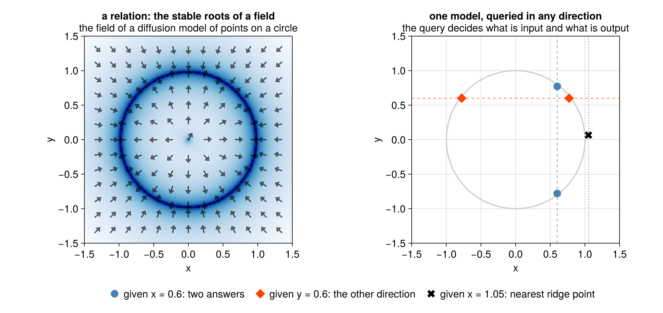
Left: the field of a diffusion model of points on a circle; it vanishes (dark) on the circle, and its stable roots are the relation. Right: the three queries of the table, answered by that one model. This is the closed-form model of the example below; tutorial 2 trains a small network and answers the same queries. (docs/readme_figure.jl draws it.)

A function cannot do any of these three things. A relation does all of them.

The analogy behind it: polynomials and varieties

The clean case that motivates every design choice. An explicit learner fits a polynomial $y=f_{\theta }(x)$; an implicit learner fits the zero set of a polynomial residual, $\{z:r_{\theta }(z)=0\}$, an algebraic variety:

aspect	explicit	implicit
approximator	functions $f_{\theta }:X\to Y$ (polynomials)	relations $R_{\theta }\subseteq Z$ (algebraic varieties)
inference	forward evaluation	root finding
backpropagation	reverse-mode automatic differentiation	the implicit function theorem
universal approximation	continuous functions on compacta (Weierstraß)	compact smooth manifolds (Nash–Tognoli)
well-posedness	always single-valued	may be multi-valued, or have no solution (then: the closest point)
loss	$\Vert f_{\theta }(x)-y{\Vert }^2$	$\Vert r_{\theta }(z){\Vert }^2$
symmetry	fixed input → output direction	no distinguished input or output
cost of inference	cheap	expensive (Newton’s method, …)
wiring	directed acyclic graph	arbitrary graph

How it works

1. A relation is the zero set of a learned residual, $R_{\theta }=\{z\in Z:r_{\theta }(z)=0\}$.
2. A query chooses a polarity: it splits the coordinates of $Z$ into inputs $X$, outputs $Y$ and latents $U$, with a precision per coordinate (∞ = hard input, 0 = free output, in between = soft evidence).
3. Inference is root-finding on the residual with the inputs clamped, the way a deep equilibrium model is evaluated.
4. Backpropagation is the implicit function theorem: one adjoint linear solve gives the gradients for the parameters, the inputs and the precisions. Nothing is unrolled.

Three model families provide the residual:

family	residual comes from	inference
diffusion models	a trained denoiser (its score)	a proximal step, or a fixed point of the denoiser
equilibrium models (DEQ, neural ODE)	a learned layer	fixed-point / root solve
algebraic (polynomials → varieties)	polynomial equations	root finding

and factor graphs wire many relations together. Where a neural network is a DAG of layers, this is an undirected graph of factors, solved by message passing (as in GTSAM, the project’s inspiration: GTSAM with learnable, non-Gaussian factors).

A minimal example

using VariationalDiffusion, LuxCore, Random
sched = VPSDE()
θ = range(0, 2π; length = 49)[1:48]
circle = NoisePredictor(GaussianMixtureEps(sched, vcat(cos.(θ)', sin.(θ)'); s = 0.05), sched)
ps, st = LuxCore.setup(Xoshiro(0), circle)            # a diffusion model of the unit circle
m = ImplicitDiffusion(circle, field_nodes(Xoshiro(1), 2; samples = 8))
 
up, _ = implicit_infer(m, [0.6,  0.5], [Inf, 0.0], ps, st)   # x clamped (∞), y free (0)
dn, _ = implicit_infer(m, [0.6, -0.5], [Inf, 0.0], ps, st)   # same query, other start
up.z[2], dn.z[2]                                              # ≈ (0.78, -0.78): two branches

The closed-form circle model is used so the example needs no training. implicit_pullback differentiates the answer, and training a relation through its own inference (a parabola learned from a circle) is worked through in the vault.

Where to go next

you are	start with
who learns by running code	the tutorials (also as Jupyter notebooks): the circle, a trained MLP, a robot arm, ProxDM, equivariant vs. conservative force fields, an energy-parametrised diffusion model, and a force law discovered from particle trajectories
from machine learning	Implicit Diffusion Learners → Backpropagation through Implicit Inference → DEQ as a Relation
from statistics / robotics	the localisation tutorial (GTSAM’s odometry example: smoothing vs filtering, noise estimated from the marginal likelihood) → Beliefs → Bethe Free Energy
from category theory	Factors are Parameterized Statistical Games, with the background in the CT-ML wiki (Track E)
looking for an API	the API documentation

The theory vault (website; also this repository opened in Obsidian, starting from vault/Start Here.md) is the larger half of the project: the derivations, the papers, the design decisions, and an honest list of what does not work yet.

What is in the repository

One umbrella package over five smaller ones. All depend on LuxCore only — not Lux, Zygote or Optimisers — so any Lux model wraps as a factor without pulling them in. Automatic differentiation and Reactant compilation come in through package extensions, for whichever backend you load.

package	gives you
LenticulumCore	what a factor is: channels, polarities, beliefs, energies
Mycelium	how factors are wired and scheduled: graphs, messages, free energy
Lenticulum	linear-Gaussian factors and Gaussian beliefs (nonlinear factors are planned)
VariationalDiffusion	diffusion models as relations: VP-SDE, RED-Diff, ProxDM, deterministic implicit inference with an adjoint backward pass
ImplicitLayers	deep equilibrium models and neural ODEs as factors
Adversarial	implicit generative models: generators and density-ratio factors

How it relates to what you know

• Lux.jl. Lenticulum builds on LuxCore and can use any Lux model. A Lux layer is a fixed forward/backward pair. A Lenticulum factor becomes one only after a query chooses its inputs, and its backward pass can be a posterior rather than a gradient.
• Deep equilibrium models / implicit layers. Same inference (root-finding) and the same backward pass (the implicit function theorem). The difference is that the direction is not fixed, and a factor carries an energy with a probabilistic reading.
• Diffusion-based inverse problems (RED-Diff, DPS). These are inference methods for one direction of the relation. Lenticulum makes the deterministic version differentiable, so the relation can be trained through its own inference.
• GTSAM / factor-graph SLAM. The same graphs and message passing, generalised to learned, non-Gaussian factors. Today the exact results are on the linear-Gaussian fragment.
• Category theory. A factor is a parameterized statistical game in the sense of AutoBayes, and a lens once a polarity is chosen; the CT-ML wiki has the background. You do not need any of it to use the code.

Using it

Not registered. From a clone:

using Pkg
Pkg.develop(path = "/path/to/Lenticulum.jl")
Pkg.develop(path = "/path/to/Lenticulum.jl/lib/VariationalDiffusion.jl")   # and the others under lib/

Tests, per package:

julia --project=.                              -e 'using Pkg; Pkg.test()'
julia --project=lib/VariationalDiffusion.jl    -e 'using Pkg; Pkg.test()'
# ... likewise for lib/LenticulumCore.jl, lib/Mycelium.jl, lib/ImplicitLayers.jl, lib/Adversarial.jl

Documentation, API and vault together:

julia --project=docs -e 'using Pkg; Pkg.instantiate()'
julia --project=docs docs/make.jl          # API docs + the vault, into docs/build/
docs/site/build.sh --serve                 # just the vault, live-previewed (Node ≥ 22)

Status and limits

A prototype. Exactness results are on the linear-Gaussian fragment and on closed-form test models. Learned networks are small by design (a factor’s joint space has a handful of coordinates, so a few-thousand-parameter MLP is enough); one is trained, queried and differentiated through its own inference in lib/VariationalDiffusion.jl/examples/circle_mlp.jl, with the AD backend chosen per model (Zygote, Enzyme, ForwardDiff, Mooncake, or Reactant for compiled XLA). Point inference returns one branch of a multivalued relation; sampling-based conditional inference is not implemented (ProxDM’s unconditional sampler is). The vault’s Related Julia Projects says what to use instead when you need only one of the things this combines.