One implicit diffusion model of (image, label) on MNIST, queried in both directions: clamp the image and the free label is a classification; clamp the label and the free image is a digit; clamp half an image and both the rest and the label come out at once. The demo of “one relation, polarity chosen at query time” that everyone recognises. Run (§6), with a split result. Image → label works: 96.1% by root finding, the same as a diffusion classifier with the same network (95.8%). Label → image does not: with this model the clamped label barely affects the generated image (8–25% of samples show the requested digit).
Sources: original to this vault (experiment design); LeCun, Bottou, Bengio & Haffner, Gradient-Based Learning Applied to Document Recognition, Proc. IEEE 1998 (MNIST); Grathwohl et al., Your Classifier is Secretly an Energy Based Model…, ICLR 2020 (JEM); Li et al., Your Diffusion Model is Secretly a Zero-Shot Classifier, ICCV 2023; Clark & Jaini, Text-to-Image Diffusion Models are Zero-Shot Classifiers, NeurIPS 2023; Bao et al., One Transformer Fits All Distributions in Multi-Modal Diffusion at Scale, ICML 2023 (UniDiffuser); Lugmayr et al., RePaint, CVPR 2022; code:
implicit.jl,answers.jl,energy_network.jlBibliography: LeCun et al. 1998 · Grathwohl et al. 2020 · Li et al. 2023 · Clark & Jaini 2023 · Bao et al. 2023 · Lugmayr et al. 2022
Theory: Implicit Diffusion Learners · Inference Signatures · Mixture Belief · Backward Signatures
1. The setup
The joint state is with the image and the label
, a one-hot vector (possibly scaled, so that the label is not drowned by
784 pixel coordinates in the denoising loss). Train ordinary denoising on the concatenation, with
an EnergyNetwork, so that answers get weights (§3). The direction is chosen only at query time,
by the precisions :
| query | clamped () | free | computed by |
|---|---|---|---|
| classify | implicit_roots / implicit_mixture on 10 coordinates | ||
| the most typical “3” | implicit_infer: a mode, §2 | ||
| draw a “3” | implicit_sample, the clamped sampler (signature #6 of Inference Signatures) | ||
| inpaint and classify | half of | the other half, and | implicit_infer |
The last row is the one no ordinary classifier or generator does, and it costs nothing extra.
2. What each direction returns
Classification is cheap: a 10-dimensional solve with a 10×10 Jacobian block. The answers
are roots near the one-hot vectors; with an energy, implicit_mixture’s Laplace-mass weights
are class probabilities, and their calibration is a
measurable result (reliability diagram against a softmax classifier). An ambiguous digit should
give two roots of comparable weight, which is the point of returning a mixture rather than an
argmax.
Generation by root finding returns a mode of the smoothed : one deterministic prototype per basin, not a sample. Whether the modes look like digits or like blurry class averages depends on the smoothing scale (the field’s noise levels, Implicit Diffusion Learners §5), and is an experiment of its own. Multi-start from noise finds several modes (styles of “7”), but with no frequencies attached unless the weights are computed in 784 dimensions.
Sampling needs the reverse SDE with the label coordinates held fixed, the replacement trick of RePaint: the same network, no retraining, but the sampler path, not the implicit solver.
3. How this differs from the prior work
| how it classifies | how it generates | |
|---|---|---|
| JEM (Grathwohl et al. 2020) | the logits of a classifier read as an energy of | SGLD on that energy |
| diffusion classifiers (Li et al. 2023; Clark & Jaini 2023) | Bayes’ rule over per-class denoising errors: one Monte-Carlo pass per class | the diffusion model itself |
| UniDiffuser (Bao et al. 2023) | one noise level per modality, every conditional from one network | the same |
| this | root finding in label space, with Laplace weights as probabilities | modes by root finding; samples by a clamped reverse SDE |
The claim worth testing is the cost line: a 10-dimensional solve against ten Monte-Carlo estimates of a denoising loss. The accuracy will most likely sit below a plain classifier’s ~99%. The selling point is one model for three queries, with uncertainty, not the benchmark.
4. Interfaces that have to exist first
- Partial Jacobians — done.
prior_jacobian(…; coords = free)computes only , and the pullback gets from one VJP (prior_vjp). On a 794-dimensional MLP with 10 free coordinates a solver iteration went from about 26 s to 0.04 s (implicit §6). - Batching and matrix-free solves (Open Problems in Implicit Diffusion Learning I5) —
done: one network call per noise level (
batched = true), andlinsolve = KrylovSolve()(GMRES, Lanczos stability, stochastic Lanczos ). With the image free (784 of 794 coordinates) a solve takes 1.1 s (krylov). Many queries at once: done,implicit_infer_manyevaluates all unfinished queries in one network call per noise level (implicit §7). - A clamped sampler for ε- and energy networks (I1) — done:
implicit_sample(m, z₀, ρ, ps, st; n, steps, resample, rng), the reverse diffusion with the hard-clamped coordinates replaced at every step and RePaint’s resampling (sampler). - A categorical answer — done:
implicit_classifystarts from every class code and reads the mixture of roots as aCategoricalBelief. The mass of roots far from every code is reported asunassigned. On three closed-form classes the probabilities are within 0.04 of the exact posterior (implicit §8). - Energy networks at this size, on a GPU — done:
device = (to = gpu_device(), back = cpu_device())withad = SecondOrder(AutoForwardDiff(), AutoZygote()). At this network size a training step takes 6 ms and a classification iteration 1.8 ms per query, in batches of 1000 (energy_network §8). Enzyme and Reactant are not needed for it. - Optional: the backward signatures (Backward Signatures), only if the generative model
is fine-tuned discriminatively through the classification query. Pure denoising training
needs none of it. The solver level is there:
Zygote.gradientdifferentiates throughimplicit_inferby itsrrule.
The data loader (MLDatasets.jl) belongs in the tutorial’s environment, never in a package’s dependencies.
Found by the experiment (§6): still needed for the generative direction and for graded answers. These are open problems I12 and I13 in Open Problems in Implicit Diffusion Learning.
- A noise level per block of coordinates (UniDiffuser) — done:
NoisePredictor(…; blocks),block_times, blocklevelson the relation, held clamps in the sampler (predictor §6, implicit §9, sampler §5). It makes label → image work (§7). - Classifier-free guidance — done (
guidance), but on this model it lowers the rate at which samples are recognised as their label (§7). Independent block times already train the unconditional score, so no separate label dropout is needed. - Loss weights per coordinate — done:
denoising_gradient(…; weights). - A class probability from a single root — done:
categorical_answer(…; temperature, cov_scale)withcalibrate_temperature; calibration error 0.009 (§7). Theunassignedmass goes tocoverage(…; unassigned)as a flag. - A globalised solver — done: the trust-region method (the default for energy relations) finds stable modes for 19 of 20 starts in about 6 s each, where Newton-or-descent found none (§7). Continuation in the noise level, tried first, reached 3–4 of 10.
- Tolerances that follow the arithmetic — done:
default_tolerance(about 1e-6 for Float32 on a device). - A convolutional energy network — done (§8–9): alone, image-like but noisy samples and a weaker classifier. With a Gaussian reference energy and training that holds a block clean as queries do, clean digits (76.5% recognised with guidance 1) and 96.8% classification from the same network.
5. What the tutorial was meant to show
Classification accuracy and calibration; the class prototypes (modes) beside samples; an ambiguous digit with a two-component answer; inpainting of the lower half of a digit together with its label; and the cost per query against a diffusion classifier with ten denoising passes.
6. The experiment (October 2026)
Code: lib/VariationalDiffusion.jl/examples/mnist/ (its own environment; logs and models in
~/.cache/lenticulum/mnist/).
The model. An energy network on : the image , the label
one-hot, 16 time features. It is an MLP 810 → 1024 → 1024 → 1024 → 1 with swish activations,
, ad = SecondOrder(AutoForwardDiff(), AutoZygote()), and runs on an RTX
3080 through device. It is trained by denoising score matching with one noise level shared by
image and label, AdamW with cosine decay, batch 256, 9 s per epoch. The label is 10 of 794
coordinates, and unweighted it barely enters the loss. Weighting its coordinates in the loss is
what made the classifier work:
| training | classification accuracy (1000 tuning images) |
|---|---|
| label weight 1, 40 epochs | 89.2% |
| label weight 20, 40 epochs | 93.4% |
| label weight 100, 100 epochs | 95.9% |
Image → label. The query clamps the 784 pixels and frees the 10 label coordinates. The field’s noise levels were chosen on test images 9001–10000: 0.002–0.05, 0.05–0.2 and 0.1–0.4 gave 95.6%, 95.9% and 94.8%. Results on test images 1–9000:
| classifier | accuracy | cost per query |
|---|---|---|
| root finding, one start, the label read as the argmax of the root | 96.1% | 18 ms (batches of 1000) |
root finding from all ten class codes (implicit_classify) | 96.1% | 220 ms |
| the diffusion classifier of Li et al., same network, 32 shared noise draws × 10 classes | 95.8% | 3.1 ms (320 network passes) |
| a softmax MLP of the same width, 10 epochs | 97.7% |
-
One answer per query. Every one of the 9000 queries has a single stable root: the ten starts all reach it. So
implicit_mixturehas one component, and its Laplace class probabilities are 0 or 1. The ten starts buy nothing, and the probabilities expected in §2 do not appear. The graded information is in where the root lies. A typical digit’s root is near its code (label coordinate about 0.8–1). For an atypical one it is between two codes:
The “2” written like an “a” is at 2: 0.49 / 3: 0.48, the 6 at 6: 0.54 / 5: 0.54. A flat “0” is at 7: 0.18 / 6: 0.18: its root is far from every code. That is the
unassignedcase ofcategorical_answer(1.1% of the test set), and an answer coverage should flag. -
Equal to the diffusion classifier, not cheaper. The two classifiers read the same network and agree in accuracy. The claim in §3 that a 10-dimensional solve beats ten Monte-Carlo estimates does not hold here. Each Newton iteration of the solve needs ten Hessian-vector products per noise level. The diffusion classifier’s 320 forward passes batch better on a GPU.
-
Both generative classifiers stay below the discriminative baseline (96 against 97.7%), as is usual for generative classifiers with small networks.
Label → image. The query clamps the label and frees the image. It fails, for two separate reasons.
-
The samples are poor. An MLP over 794 joint coordinates gives noisy digits. With the energy parametrisation they are noisier than with an ε-network of the same size; a few are clean.
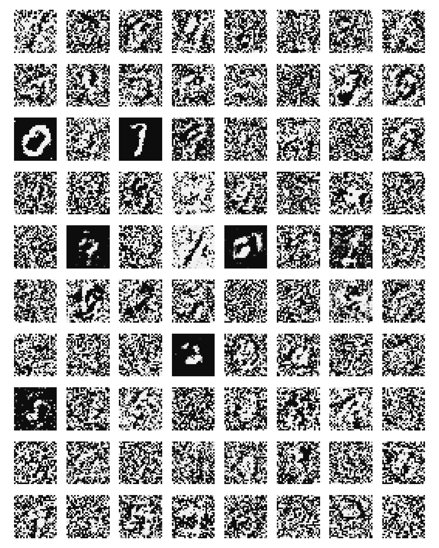
-
The label hardly conditions the image. 20 samples per class were scored by a softmax MLP trained on real data (chance 10%):
model plain RePaint ×3 Langevin ×2 both label held clean at every step ε-network 11.5% 10.0% 12.5% 12.5% 13.0% energy, label weight 1 7.5% 13.0% 17.5% 16.0% energy, label weight 100 11.0% 25.0% 16.5% 21.0% 16.5% Holding the label clean instead of noising it does not help, so this is not the replacement method losing the label to noise. The network’s score for the image barely depends on the label. In the joint score, , the second term is small next to the image’s own structure, and nothing in the training makes the network resolve it. The label’s score does depend on the image, which is why classification works. The relation is learned well in one direction only.
Mode finding in the image (784 free, KrylovSolve) did not converge from a blank image or
from a sample: the solve leaves the sample (1.7 to 6 per pixel, RMS) and ends unstable. The
smoothed energy of this model has no usable basins in image space at the field’s noise levels.
Inpainting with the label free was therefore not run.
What this says about the method. Classification as a query works at the accuracy of the established diffusion classifier, with a single generic solver, and its failure cases are visible: roots between the codes. Generation from the same relation needs what the text-to-image literature already found necessary:
- classifier-free guidance, which needs training with the label dropped;
- separate noise levels per block, as in UniDiffuser, so that a clean label can condition a noisy image;
- a convolutional energy for image quality.
The first two are changes to the training and the sampler, not to the query machinery. The second needs a noise level per block of coordinates, which the package did not have; §7 adds it.
7. With a noise level per block (October 2026)
The same network and training, except that image and label are two noise blocks
(blocks = [1:784, 785:794], 32 time features), each trained at its own time drawn from
(block_times; 20% of each batch with one shared time), label weight 100,
100 epochs (BLOCKS=1 MODEL=blocks_w100). A query holds its clamped block clean and anneals the
free one (conditional_levels, clamp_level).
Label → image now uses the label. 20 samples per class, scored by the same softmax judge (chance 10%):
| sampler, same block-trained network | recognised as the clamped label | mean judge probability |
|---|---|---|
label held clean (clamp_level = tmin) | 85.5% | 0.852 |
| held, guidance 1 | 74.0% | 0.736 |
| held, guidance 3 | 71.5% | 0.711 |
| label replaced by its forward marginal (as in §6) | 10.5% | 0.110 |
Training with independent block times alone is not enough. With the label replaced, as the old sampler did, the same network is at chance. Holding the label clean was tried on the old network in §6 and did not help, because that network had never seen a clean label beside a noisy image. It is the combination that conditions: a network trained on every pair of levels, and a sampler that gives it the clamp clean. Guidance, the usual remedy, makes it worse here.
The images are still not good digits. The judge picks up label-specific structure, but the samples are mostly noise; the old model’s few clean digits do not reappear:
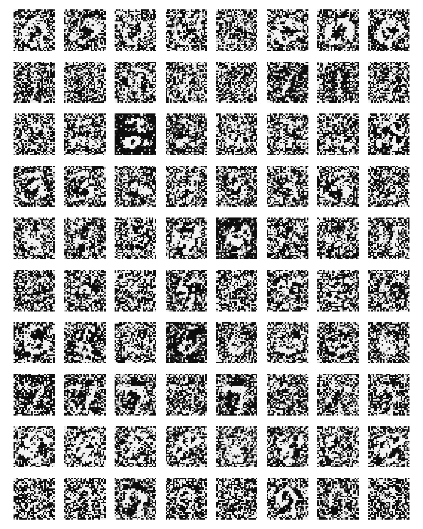
The bottleneck is the image score of an MLP energy over 794 coordinates (item 13), not the conditioning; §9 locates it at high noise and in the held condition’s training.
Image → label, held against joint. One start, argmax of the root, tuning images 9001–10000, same network:
| field levels | image held clean | joint field (image noised too) |
|---|---|---|
| 0.002–0.05 | 93.9% | 93.7% |
| 0.05–0.2 | 95.0% | 94.0% |
| 0.1–0.4 | 95.3% | 93.1% |
| 0.02–0.5 | 95.0% | 92.6% |
Holding the image clean matters more the more the field smooths, as on the circle (implicit §9). But the block-trained network classifies slightly worse than the joint-only network of §6: 95.3% against 95.9% on the tuning images, and on test images 1–3000 (mid levels) 92.6% against 94.6%. One network for both directions costs about one to two points here.
Class probabilities from single roots. Every query again has one stable root. Reading the
root’s Laplace Gaussian as evidence about the code (categorical_answer(…; temperature, cov_scale)), fitted on the tuning images and scored on test images 1–3000 (mid levels, ten
starts):
| reading | accuracy | NLL | calibration error (ECE) | mean max-probability |
|---|---|---|---|---|
| Laplace weights, hard assignment | 90.3% | 1.459 | 0.052 | 0.955 |
| code posterior, τ only (τ at its bound 0.001) | 92.5% | 0.509 | 0.250 | 0.675 |
| code posterior, τ = 0.001 and κ = 0.45 | 92.5% | 0.244 | 0.009 | 0.926 |
| softmax MLP (§6, test images 1–9000) | 97.7% | 0.011 |
The Laplace covariance at density_lambda is about twice too wide (κ = 0.45 shrinks it), so a
temperature alone, which can only widen it, makes the answers underconfident. With κ the root’s
position gives calibrated probabilities, as calibrated as the discriminative baseline’s, at its
lower accuracy. The hard reading loses the 2% of roots that lie between codes.
A factor of about two is what the nodes’ noise predicts: averaging the log-density over the
nodes’ shifts smooths a second time (Implicit Diffusion Learners §5), so the potential’s
curvature is that of a density smoothed twice. This is a conjecture for this model: it has not
been checked here by repeating the fit with noisefree_nodes.
Modes with the label held (784 free coordinates, KrylovSolve, 50 iterations per stage):
| start | continuation | converged and stable | judged as the label | median residual | time per mode |
|---|---|---|---|---|---|
| blank image | none | 0/10 | 5/10 | 2.9 | 25 s |
| blank image | (8, 3) | 3/10 | 8/10 | 1.4 | 221 s |
| a sample | none | 0/10 | 8/10 | 16 | 19 s |
| a sample | (8, 3) | 4/10 | 8/10 | 0.48 | 123 s |
Continuation in the noise level helps the solver into basins, but at five to nine times the cost and still converging in fewer than half the cases. The trust-region solver (implicit §11), on the same queries:
| start | converged and stable | judged as the label | median residual | iterations | time per mode |
|---|---|---|---|---|---|
| blank image | 10/10 | 6/10 | 16 | 6 s | |
| a sample | 9/10 | 9/10 | 37 | 6 s |
Cost against the diffusion classifier (cost.jl, implicit §12). On this model one-start
root finding takes 15.1 ms per query (Newton-or-descent) or 18.5 ms (trust region) at 95.0%, the
diffusion classifier 3.1 ms at 93.9% with 32 draws, and more draws do not raise its accuracy
(94.2% at 128, 93.7% at 256). A pass-count model predicts the ratio within 10%. Root finding pays
mostly for the Jacobian block, ten Hessian-vector products per node and iteration; with
one-hot labels that grows with the classes, so it is never the cheaper method here.
Every converged mode is a stable minimum of the query’s energy. That several are judged as another digit (an 8 most often) is the model’s mode, not the solver’s: the most probable image of an MLP energy given a label need not look like a typical sample of it.
8. A convolutional energy (October 2026)
KIND=conv: the image through three 3×3 convolutions (28 → 14 → 7 pixels, 32 → 64 → 64 channels),
the time features of both blocks and the label added as per-channel biases after each
convolution and given to a dense head, which returns the scalar energy; 877k parameters. Same
training as §7 (noise blocks, label weight 100, 100 epochs). Its second derivatives run as for
the MLP, ForwardDiff over Zygote on the GPU: LuxLib passes dual numbers through cuDNN
convolutions; Zygote over Zygote does not. A training step takes 23 ms (6 s per epoch, faster
than the MLP); a batched Jacobian block of 1000 queries does not fit in 10 GB, so queries go in
chunks of 100 (CHUNK).
Label → image (20 samples per class, the same judge):
| sampler | MLP energy (§7) | conv energy | conv, stopped at t = 0.03 |
|---|---|---|---|
| label held clean | 85.5% | 31.0% | 29.0% |
| held, guidance 1 | 74.0% | 42.5% | 46.0% |
| held, guidance 3 | 71.5% | 27.5% | 29.5% |
| label replaced | 10.5% | 11.5% | 10.0% |
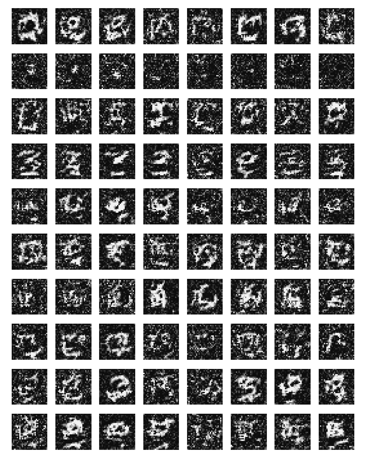
The samples look more like MNIST than the MLP’s: dark backgrounds, strokes, some legible 0s, 3s and 9s. They are recognised less often, because the MLP’s noise carried label-specific structure that its judge picked up, and the conv model’s conditioning is weaker (guidance now helps, by 11 points). Both are still covered in pixel noise.
The error per noise level. The image’s ε error per pixel, label held clean, on 500 test images:
| t (σ) | 0.001 (0.01) | 0.003 (0.02) | 0.01 (0.045) | 0.03 (0.11) | 0.1 (0.32) | 0.3 (0.78) | 0.7 (1.0) |
|---|---|---|---|---|---|---|---|
| MLP energy | 0.997 | 0.992 | 0.948 | 0.744 | 0.284 | 0.100 | 0.046 |
| conv energy | 0.971 | 0.902 | 0.574 | 0.322 | 0.167 | 0.102 | 0.044 |
At low noise both predict almost nothing (an error of 1 is ε = 0), though about 80% of MNIST pixels are exactly background and their noise is recoverable. This section first took that for the cause of the noisy samples. It is not: an ε error of 1 at σ = 0.02 leaves a pixel error of 0.02, which is invisible. §9 finds the cause at the other end of the noise range, and a fix.
Two parametrisations aimed at the low-noise end were tried first and dropped:
- the energy divided by the image block’s σ, : error 0.92 at the lowest level instead of 0.97, recognition 36%; no visible change;
- a denoiser energy, with , which has the right curvature by construction. With the last layers at zero it does not train at all (U and its Jacobian vanish together, and with them the loss gradient); with a small random start its loss stayed above 1 after 17 epochs (the scalar conv energy was at 0.15 after 7) and it was stopped.
Image → label (one start, tuning images, default tolerance): 92.8% at levels 0.05–0.2 with 96% of the solves converged, at 421 ms per query, against 95.0% at 17 ms for the MLP. Each Jacobian block needs ten Hessian-vector products through the convolutions, in chunks of 100 queries.
So the convolutions improve the images’ structure but not their noise, and cost the classifier.
9. Where the noise came from, and a fix (October 2026)
Where. denoise_eval.jl noises 50 test images to a level t₀ (label held clean), runs the
sampler’s steps from there down to and counts the pixels of the 3-pixel border,
background in every digit, that end brighter than −0.5:
| border speckles, started at t₀ (σ) | 0.1 (0.32) | 0.3 (0.78) | 0.5 (0.96) | 1.0 (1.0) |
|---|---|---|---|---|
| MLP energy (§7) | 0.7% | 1.3% | 13.6% | 48.7% |
| conv energy (§8) | 1.0% | 9.0% | 16.3% | 18.6% |
| conv energy with the reference energy | 0.4% | 0.3% | 0.4% | 1.7% |
| … and clean blocks in training, held block out of the loss | 0.3% | 0.2% | 0.2% | 0.2% |
From a real image noised to 0.1 both energies come back almost clean; the speckles come from the part of the reverse diffusion above t ≈ 0.3. There the denoised estimate is with up to 150, and an ε error that looks small (0.044 at t = 0.7) is a large error in the image: the Gaussian below has 0.002 there.
Two causes.
- The energy has to build the Gaussian part itself. At high noise the score is almost that of a
Gaussian, an energy -like over 794 coordinates, and the networks get it
wrong.
REF=1adds the exact energy of a diagonal Gaussian fitted to the data, , and the network learns the rest. A pixel that is background in every training image () gets curvature from it at every level. - Training never sees the condition the sampler uses. The sampler holds the label clean; block
times uniform on give a label that clean in about 1% of the columns. On the MLP
with the reference, the image’s ε error at t = 0.7 is 0.002 with the label noised with the image
and 0.073 with it held clean (0.027 against 0.047 for the MLP of §7).
block_times(…; clean)holds one block, chosen at random, at in the given fraction of the columns, andHELD_LOSS=0leaves that block out of the loss: it is a condition there, not a target.
Result (conv energy, REF=1 CLEAN=0.5 HELD_LOSS=0, otherwise as §8). The ε error per pixel:
| t (σ) | 0.001 (0.01) | 0.003 (0.02) | 0.01 (0.045) | 0.03 (0.11) | 0.1 (0.32) | 0.3 (0.78) | 0.7 (1.0) |
|---|---|---|---|---|---|---|---|
| conv energy (§8) | 0.971 | 0.902 | 0.574 | 0.322 | 0.167 | 0.102 | 0.044 |
| with the reference and clean blocks | 0.836 | 0.754 | 0.519 | 0.227 | 0.096 | 0.050 | 0.002 |
Label → image, 20 samples per class, the same judge:
| sampler | MLP energy (§7) | conv (§8) | conv, reference | … clean blocks | … held block out of the loss |
|---|---|---|---|---|---|
| label held clean | 85.5% | 31.0% | 21.0% | 37.0% | 49.0% |
| held, guidance 1 | 74.0% | 42.5% | 15.0% | 72.0% | 76.5% |
| held, guidance 3 | 71.5% | 27.5% | 12.0% | 60.0% | 71.5% |
| label replaced | 10.5% | 11.5% | 12.5% | 11.0% | 10.5% |
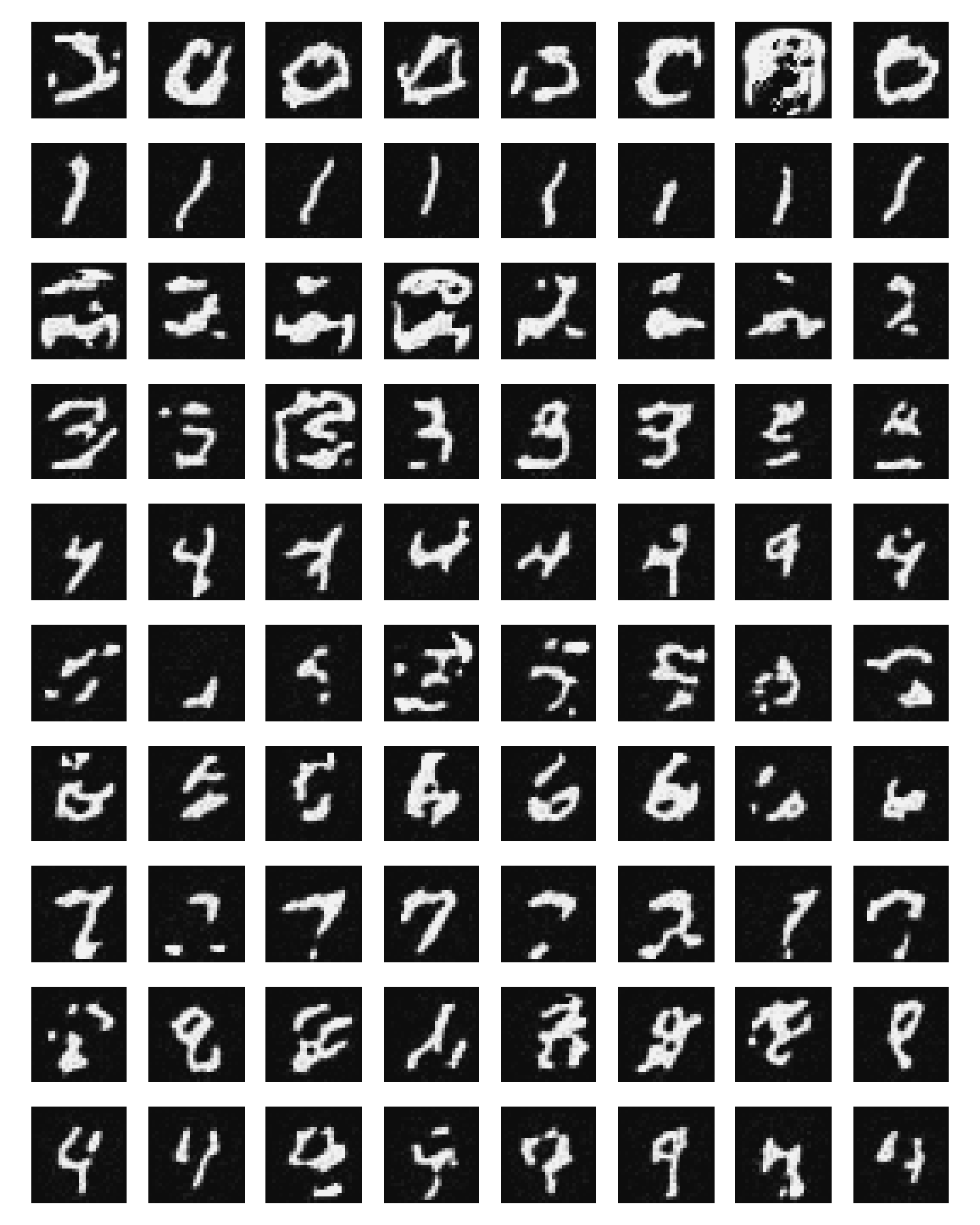
The samples are digits on a clean background, with strokes and no pixel noise; most are legible. The MLP of §7 scores higher on the judge with images that are mostly noise: the judge reads label-specific structure in the noise, so its rate is not a measure of image quality.
Image → label with the same network (one start, levels 0.05–0.2, the 1000 tuning images, default tolerance): 96.8%, 94% of the solves converged, 291 ms per query in chunks of 50. That is above the MLP energy of §7 (95.0%) and the conv energy of §8 (92.8%): the clean blocks train the classifier’s condition too, where the image is held clean.
On the 9000 test images (1–9000), the same reading: 96.6%, 96.5% of the solves converged and stable (97.3% correct among those, 77% among the rest), 396 ms per query in chunks of 100 (the GPU shared with other jobs for part of the run). That is above the first MLP energy (96.1%) and the diffusion classifier with its network (95.8%), and below the softmax MLP (97.7%).
Its class probabilities, read as in §7 (ten starts, mid levels, τ and κ fitted on the 1000 tuning images, scored on test images 1–1000; 2.1 s per query in chunks of 5):
| reading | accuracy | NLL | calibration error (ECE) | mean max-probability |
|---|---|---|---|---|
| Laplace weights, hard assignment | 95.8% | 0.909 | 0.036 | 0.990 |
| code posterior, τ only (τ at its bound 0.001) | 96.1% | 0.279 | 0.145 | 0.821 |
| code posterior, τ = 0.001 and κ = 0.57 | 96.1% | 0.154 | 0.015 | 0.970 |
The pattern of §7 holds: the Laplace covariance is too wide (κ = 0.57 shrinks it), a temperature alone makes the answers underconfident, and with κ they are calibrated (ECE 0.015 against 0.009 for the MLP of §7, on fewer test images), at higher accuracy and with a lower NLL (0.154 against 0.244). 98.8% of the tuning queries have one root.
What does not work. The reference needs the convolutions. On the MLP every sample falls into
one spurious image, the same for every label (10% recognised), with or without clean blocks; the
MLP with clean blocks and no reference keeps its speckles (48% from t₀ = 1, 19–29% recognised).
The reference is a package option, EnergyNetwork(net; reference = GaussianReference(X)), with its
derivatives in closed form (energy_network.md §9). It gives this model the same denoising errors
and samples as the first version, which had it inside the network and differentiated it by AD.
Related: Implicit Diffusion Learners, Inference Signatures, Composing Diffusion Factors, Open Problems in Implicit Diffusion Learning, Language Models, Motivating Examples